This post is a numpyro-based probabilistic model of my blood glucose data (see my original blogpost for necessary background).
The task is, given my blood glucose readings, my heart rate data, and what I ate,
can I figure out the contribution of each food to my blood glucose.
This is a classic Bayesian problem, where I have some observed data (blood glucose readings),
a model for how food and heart rate influence blood glucose,
and I want to find likely values for my parameters.
Normally I would use pymc3 for this kind of thing, but this was a good excuse to try out numpyro, which is built on JAX,
the current favorite for automatic differentiation.
To make the problem a little more concrete,
say your fasting blood glucose is 80, then you eat something and an hour later it goes to 120,
and an hour after that it's back down to 90. How much blood glucose can I attribute to that food?
What if I eat the same food on other day, but this time my blood glucose shoots to 150?
What if I eat something else 30 minutes after eating this food so the data overlap?
In theory, all of these situations can be modeled in a fairly simple probabilistic model.
Imports
I am using numpyro, and jax numpy instead of regular numpy.
In most cases, jax is a direct replacement for numpy, but sometimes I need original numpy, so I keep that as onp.
#!pip install numpyro
import jax.numpy as np
from jax import random
from jax.scipy.special import logsumexp

import numpyro
import numpyro.distributions as dist
from numpyro.diagnostics import hpdi
from numpyro import handlers
from numpyro.infer import MCMC, NUTS

import numpy as onp
import seaborn as sns
import pandas as pd
import matplotlib.pyplot as plt

import glob
import json
import io

from tqdm.autonotebook import tqdm
from contextlib import redirect_stdout

%config InlineBackend.figure_format='retina'
Some simple test data
Simple test data is always a good idea for any kind of probabilistic model.
If I can't make the model work with the simplest possible data,
then it's best to figure that out early, before starting to try to use real data.
I believe McElreath advocates for something similar, though I can't find a citation for this.
To run inference with my model I need three 1D arrays:
bg_5min: blood glucose readings, measured every 5 minuteshr_5min: heart rate, measured every 5 minutesfd_5min: food eaten, measured every 5 minutes
def str_to_enum(arr):
    foods = sorted(set(arr))
    assert foods[0] == '', f"{foods[0]}"
    mapk = {food:n for n, food in enumerate(foods)}
    return np.array([mapk[val] for val in arr]), foods

bg_5min_test = np.array([91, 89, 92, 90, 90, 90, 88, 90, 93, 90,
                         90, 100, 108, 114.4, 119.52, 123.616, 126.89, 119.51, 113.61, 108.88, 105.11,
                         102.089, 99.67, 97.73, 96.18, 94.95, 93.96, 93.16, 92.53, 92.02, 91.62, 91.29, 91.03, 90.83, 90.66, 90.53,
                         90, 90, 90, 90, 90, 90, 90, 89, 90, 90, 89, 90, 90, 90, 90, 90, 90, 90, 90, 95, 95, 95, 95, 100])

_fd_5min_test = ['', '', '', '', '', 'food', '', '', '', '', '', '',
                 '', '', '', '', '', '', '', '', '', '', '', '',
                 '', '', '', '', '', '', '', '', '', '', '', '',
                 '', '', '', '', 'doof', '', '', '', '', '', '', '',
                 '', '', '', '', '', '', '', '', '', '', '', '', '']

fd_5min_test, fd_5min_test_key = str_to_enum(_fd_5min_test)
hr_5min_test = np.array([100] * len(bg_5min_test))

bg_5min_test = np.tile(bg_5min_test, 1)
fd_5min_test = np.tile(fd_5min_test, 1)
hr_5min_test = np.tile(hr_5min_test, 1)

print(f"Example test data (len {len(bg_5min_test)}):")
print("bg", bg_5min_test[:6])
print("heart rate", hr_5min_test[:6])
print("food as enum", fd_5min_test[:6])

assert len(bg_5min_test) == len(hr_5min_test) == len(fd_5min_test)
Example test data (len 60):
bg [91. 89. 92. 90. 90. 90.]
heart rate [100 100 100 100 100 100]
food as enum [0 0 0 0 0 2]
Read in real data as a DataFrame
I have already converted all my Apple Health data to csv.
Here I process the data to include naive day and date (local time) — timezones are impossible otherwise.
df_complete = pd.DataFrame()

for f in glob.glob("HK*.csv"):
    _df = (pd.read_csv(f, sep=';', skiprows=1)
             .assign(date = lambda df: pd.to_datetime(df['startdate'].apply(lambda x:x[:-6]),
                                                      infer_datetime_format=True))
             .assign(day = lambda df: df['date'].dt.date,
                     time = lambda df: df['date'].dt.time)
          )

    if 'unit' not in _df:
        _df['unit'] = _df['type']
    df_complete = pd.concat([df_complete, _df[['type', 'sourcename', 'unit', 'day', 'time', 'date', 'value']]])

# clean up the names a bit and sort
df_complete = (df_complete.assign(type = lambda df: df['type'].str.split('TypeIdentifier', expand=True)[1])
                          .sort_values(['type', 'date']))
df_complete.sample(4)
I can remove a bunch of data from the complete DataFrame.
df = (df_complete
        .loc[lambda r: ~r.type.isin({"HeadphoneAudioExposure", "BodyMass", "UVExposure", "SleepAnalysis"})]
        .loc[lambda r: ~r.sourcename.isin({"Brian Naughton’s iPhone", "Strava"})]
        .loc[lambda r: r.date >= min(df_complete.loc[lambda r: r.sourcename == 'Connect'].date)]
        .assign(value = lambda df: df.value.astype(float)))
df.groupby(['type', 'sourcename']).head(1)
| type |
sourcename |
unit |
day |
time |
date |
value |
| ActiveEnergyBurned |
Connect |
kcal |
2018-07-08 |
21:00:00 |
2018-07-08 21:00:00 |
8.00 |
| BasalEnergyBurned |
Connect |
kcal |
2018-07-08 |
21:00:00 |
2018-07-08 21:00:00 |
2053.00 |
| BloodGlucose |
Dexcom G6 |
mg/dL |
2020-02-24 |
22:58:54 |
2020-02-24 22:58:54 |
111.00 |
| DistanceWalkingRunning |
Connect |
mi |
2018-07-08 |
21:00:00 |
2018-07-08 21:00:00 |
0.027 |
| FlightsClimbed |
Connect |
count |
2018-07-08 |
21:00:00 |
2018-07-08 21:00:00 |
0.00 |
| HeartRate |
Connect |
count/min |
2018-07-01 |
18:56:00 |
2018-07-01 18:56:00 |
60.00 |
| RestingHeartRate |
Connect |
count/min |
2019-09-07 |
00:00:00 |
2019-09-07 00:00:00 |
45.00 |
| StepCount |
Connect |
count |
2018-07-01 |
19:30:00 |
2018-07-01 19:30:00 |
33.00 |
I have to process my food data separately, since it doesn't come from Apple Health.
The information was just in a Google Sheet.
df_food = (pd.read_csv("food_data.csv", sep='\t')
             .astype(dtype = {"date":"datetime64[ns]", "food": str})
             .assign(food = lambda df: df["food"].str.split(',', expand=True)[0] )
             .loc[lambda r: ~r.food.isin({"chocolate clusters", "cheese weirds", "skinny almonds", "asparagus"})]
             .sort_values("date")
            )
df_food.sample(4)
| date |
food |
| 2020-03-03 14:10:00 |
egg spinach on brioche |
| 2020-03-11 18:52:00 |
lentil soup and bread |
| 2020-02-27 06:10:00 |
bulletproof coffee |
| 2020-03-02 06:09:00 |
bulletproof coffee |
For inference purposes, I am rounding everything to the nearest 5 minutes.
This creates the three arrays the model needs.
_df_food = (df_food
              .assign(rounded_date = lambda df: df['date'].dt.round('5min'))
              .set_index('rounded_date'))

_df_hr = (df.loc[lambda r: r.type == 'HeartRate']
            .assign(rounded_date = lambda df: df['date'].dt.round('5min'))
            .groupby('rounded_date')
            .mean())

def get_food_at_datetime(datetime):
    food = (_df_food
              .loc[datetime - pd.Timedelta(minutes=1) : datetime + pd.Timedelta(minutes=1)]
              ['food'])

    if any(food):
        return sorted(set(food))[0]
    else:
        return None

def get_hr_at_datetime(datetime):
    hr = (_df_hr
            .loc[datetime - pd.Timedelta(minutes=1) : datetime + pd.Timedelta(minutes=1)]
            ['value'])
    if any(hr):
        return sorted(set(hr))[0]
    else:
        return None


df_5min = \
(df.loc[lambda r: r.type == "BloodGlucose"]
   .loc[lambda r: r.date >= pd.datetime(2020, 2, 25)]
   .assign(rounded_date = lambda df: df['date'].dt.round('5min'),
           day = lambda df: df['date'].dt.date,
           time = lambda df: df['date'].dt.round('5min').dt.time,
           food = lambda df: df['rounded_date'].apply(get_food_at_datetime),
           hr = lambda df: df['rounded_date'].apply(get_hr_at_datetime)
          )
)


bg_5min_real = onp.array(df_5min.pivot_table(index='day', columns='time', values='value').interpolate('linear'))
hr_5min_real = onp.array(df_5min.pivot_table(index='day', columns='time', values='hr').interpolate('linear'))
fd_5min_real = onp.array(df_5min.fillna('').pivot_table(index='day', columns='time', values='food', aggfunc=lambda x:x).fillna('')).astype(str)
assert bg_5min_real.shape == hr_5min_real.shape == fd_5min_real.shape, "array size mismatch"

print(f"Real data (len {bg_5min_real.shape}):")
print("bg", bg_5min_real[0][:6])
print("hr", hr_5min_real[0][:6])
print("food", fd_5min_real[0][:6])
Real data (len (30, 288)):
bg [102. 112. 114. 113. 112. 111.]
hr [50.33333333 42.5        42.66666667 43.         42.66666667 42.5       ]
food ['' '' '' '' '' '']
numpyro model
The model is necessarily pretty simple, given the amount of data I have to work with.
Note that I use "g" as a shorthand for mg/dL, which may be confusing.
The priors are:
baseline_mu:
I have a uniform prior on my "baseline" (fasting) mean blood glucose level.
If I haven't eaten, I expect my blood glucose to be distributed around this value.
This is a uniform prior from 80–110 mg/dL.all_food_g_5min_mu:
Each food deposits a certain number of mg/dL of sugar into my blood every 5 minutes.
This is a uniform prior from 8–16 mg/dL per 5 minutes.all_food_duration_mu:
Each food only starts depositing glucose after a delay for digestion and absorption.
This is a uniform prior from 45–100 minutes.all_food_g_5min_mu:
Food keeps depositing sugar into my blood for some time.
Different foods may be quick spikes of glucose (sugary) or slow release (fatty).
This is a uniform prior from 25–50 minutes.regression_rate:
The body regulates glucose by releasing insulin,
which pulls blood glucose back to baseline at a certain rate.
I allow for three different rates, depending on my heart rate zone.
Using this simple model, the higher the blood glucose, the more it regresses, so it produces a
somewhat bell-shaped curve.
Using uniform priors is really not best practices, but it makes it easier to keep values in a reasonable range.
I did experiment with other priors, but settled on this after failing to keep my posteriors to reasonable values.
As usual, explaining the priors to the model is like asking for a wish from an obtuse genie.
This is a common problem with probabilistic models, at least for me.
The observed blood glucose is then a function that uses this approximate logic:
for t in all_5_minute_increments:
  blood_glucose[t] = baseline[t] # blood glucose with no food
  for food in foods:
    if t - time_eaten[food] > food_delays[food]: # then the food has started entering the bloodstream
      if t - (time_eaten[food] + food_delays[food]) < food_duration[food]: # then food is still entering the bloodstream
        blood_glucose[t] += food_g_5min[food]

  blood_glucose[t] = blood_glucose[t] - (blood_glucose[t] - baseline[t]) * regression_rate[heart_rate_zone_at_time(t)]
This model has some nice properties:
- every food has only three parameters: the delay, the duration, and the mg/dL per 5 minutes.
The total amount of glucose (loosely defined) can be easily calculate by multiplying
food_duration * food_g_5_min.
- the model only has two other parameters: the baseline glucose, and regression rate
MAX_TIMEPOINTS = 70 # effects are modeled 350 mins into the future only
DL = 288 # * 5 minutes = 1 day
SUB = '' # or a number, to subset
DAYS = [11]

%%time
def model(bg_5min, hr_5min, fd_5min, fd_5min_key):

    def zone(hr):
        if hr < 110: return "1"
        elif hr < 140: return "2"
        else: return "3"

    assert fd_5min_key[0] == '', f"{fd_5min_key[0]}"
    all_foods = fd_5min_key[1:]

    # ----------------------------------------------

    baseline_mu = numpyro.sample('baseline_mu', dist.Uniform(80, 110))

    all_food_g_5min_mu = numpyro.sample("all_food_g_5min_mu", dist.Uniform(8, 16))
    food_g_5mins = {food : numpyro.sample(f"food_g_5min_{food}",
                                          dist.Uniform(all_food_g_5min_mu-8, all_food_g_5min_mu+8))
                    for food in all_foods}

    all_food_duration_mu = numpyro.sample(f"all_food_duration_mu", dist.Uniform(5, 10))
    food_durations = {food : numpyro.sample(f"food_duration_{food}",
                                            dist.Uniform(all_food_duration_mu-3, all_food_duration_mu+3))
                      for food in all_foods}

    regression_rate = {zone : numpyro.sample(f"regression_rate_{zone}", dist.Uniform(0.7, 0.96))
                       for zone in "123"}

    all_food_delay_mu = numpyro.sample("all_food_delay_mu", dist.Uniform(9, 20))
    food_delays = {food : numpyro.sample(f"food_delay_{food}", dist.Uniform(all_food_delay_mu-4, all_food_delay_mu+4))
                   for food in all_foods}

    food_g_totals = {food : numpyro.deterministic(f"food_g_total_{food}", food_durations[food] * food_g_5mins[food])
                     for food in all_foods}

    result_mu = [0 for _ in range(len(bg_5min))]
    for j in range(1, len(result_mu)):
        if fd_5min[j] == 0:
            continue

        food = fd_5min_key[fd_5min[j]]
        for _j in range(min(MAX_TIMEPOINTS, len(result_mu)-j)):
            result_mu[j+_j] = numpyro.deterministic(
                f"add_{food}_{j}_{_j}",
                (result_mu[j+_j-1] * regression_rate[zone(hr_5min[j+_j])]
                 + np.where(_j > food_delays[food],
                            np.where(food_delays[food] + food_durations[food] - _j < 0, 0, 1) * food_g_5mins[food],
                            0)
                )
            )


    for j in range(len(result_mu)):
        result_mu[j] = numpyro.deterministic(f"result_mu_{j}", baseline_mu + result_mu[j])

    # observations
    obs = [numpyro.sample(f'result_{i}', dist.Normal(result_mu[i], 5), obs=bg_5min[i])
           for i in range(len(result_mu))]

def make_model(bg_5min, hr_5min, fd_5min, fd_5min_key):
    from functools import partial
    return partial(model, bg_5min, hr_5min, fd_5min, fd_5min_key)
Sample and store results
Because the process is slow, I usually only run one day at at time,
and store all the samples in json files.
It would be much better to run inference on all days simultaneously,
especially since I have data for the same food on different days.
Unfortunately, this turned out to take way too long.
assert len(bg_5min_real.ravel())/DL == 30, len(bg_5min_real.ravel())/DL

for d in DAYS:
    print(f"day {d}")
    bg_5min = bg_5min_real.ravel()[int(DL*d):int(DL*(d+1))]
    hr_5min = hr_5min_real.ravel()[int(DL*d):int(DL*(d+1))]
    _fd_5min = fd_5min_real.ravel()[int(DL*d):int(DL*(d+1))]
    fd_5min, fd_5min_key = str_to_enum(_fd_5min)

    #
    # subset it for testing
    #
    if SUB != '':
        bg_5min, hr_5min, fd_5min = bg_5min[-SUB*3:-SUB*1], hr_5min[-SUB*3:-SUB*1], fd_5min[-SUB*3:-SUB*1]

    open(f"bg_5min_{d}{SUB}.json",'w').write(json.dumps(list(bg_5min)))
    open(f"hr_5min_{d}{SUB}.json",'w').write(json.dumps(list(hr_5min)))
    open(f"fd_5min_key_{d}{SUB}.json",'w').write(json.dumps(fd_5min_key))
    open(f"fd_5min_{d}{SUB}.json",'w').write(json.dumps([int(ix) for ix in fd_5min]))

    rng_key = random.PRNGKey(0)
    rng_key, rng_key_ = random.split(rng_key)
    num_warmup, num_samples = 500, 5500

    kernel = NUTS(make_model(bg_5min, hr_5min, fd_5min, fd_5min_key))
    mcmc = MCMC(kernel, num_warmup, num_samples)
    mcmc.run(rng_key_)
    mcmc.print_summary()
    samples_1 = mcmc.get_samples()
    print(d, sorted([(float(samples_1[food_type].mean()), food_type) for food_type in samples_1 if "total" in food_type], reverse=True))
    print(d, sorted([(float(samples_1[food_type].mean()), food_type) for food_type in samples_1 if "delay" in food_type], reverse=True))
    print(d, sorted([(float(samples_1[food_type].mean()), food_type) for food_type in samples_1 if "duration" in food_type], reverse=True))

    open(f"samples_{d}{SUB}.json", 'w').write(json.dumps({k:[round(float(v),4) for v in vs] for k,vs in samples_1.items()}))

    print_io = io.StringIO()
    with redirect_stdout(print_io):
        mcmc.print_summary()
    open(f"summary_{d}{SUB}.json", 'w').write(print_io.getvalue())
day 11


sample: 100%|██████████| 6000/6000 [48:58<00:00,  2.04it/s, 1023 steps of size 3.29e-04. acc. prob=0.81]


                                             mean       std    median      5.0%     95.0%     n_eff     r_hat
                      all_food_delay_mu     10.39      0.29     10.40      9.95     10.86     10.32      1.04
                   all_food_duration_mu      9.22      0.20      9.22      8.93      9.51      2.77      2.28
                     all_food_g_5min_mu      9.81      0.37      9.78      9.16     10.32      5.55      1.44
                            baseline_mu     89.49      0.37     89.47     88.89     90.09      9.89      1.00
          food_delay_bulletproof coffee      7.59      0.86      7.51      6.37      8.98     23.44      1.02
      food_delay_egg spinach on brioche     13.75      0.41     13.92     13.04     14.26      4.81      1.08
              food_delay_milk chocolate      6.70      0.21      6.74      6.38      7.00     17.39      1.00
     food_delay_vegetables and potatoes     12.03      0.93     12.15     10.52     13.44     16.36      1.08
       food_duration_bulletproof coffee      9.92      1.36      9.72      8.27     12.09      2.72      2.68
   food_duration_egg spinach on brioche     11.42      0.34     11.42     10.94     11.93      2.51      2.59
           food_duration_milk chocolate      7.01      0.22      6.98      6.58      7.34     16.01      1.00
  food_duration_vegetables and potatoes      8.56      1.40      8.52      6.55     10.43      4.89      1.37
         food_g_5min_bulletproof coffee      2.45      0.38      2.41      1.86      3.01      7.07      1.58
     food_g_5min_egg spinach on brioche      7.38      0.33      7.39      6.86      7.92      9.65      1.36
             food_g_5min_milk chocolate     11.38      0.38     11.40     10.70     11.94     21.69      1.06
    food_g_5min_vegetables and potatoes     14.46      2.99     15.55      9.90     18.17     10.31      1.17
                      regression_rate_1      0.93      0.00      0.93      0.92      0.93     24.68      1.04
                      regression_rate_2      0.74      0.03      0.73      0.71      0.78      3.68      1.69
                      regression_rate_3      0.78      0.03      0.77      0.73      0.82      4.28      1.60
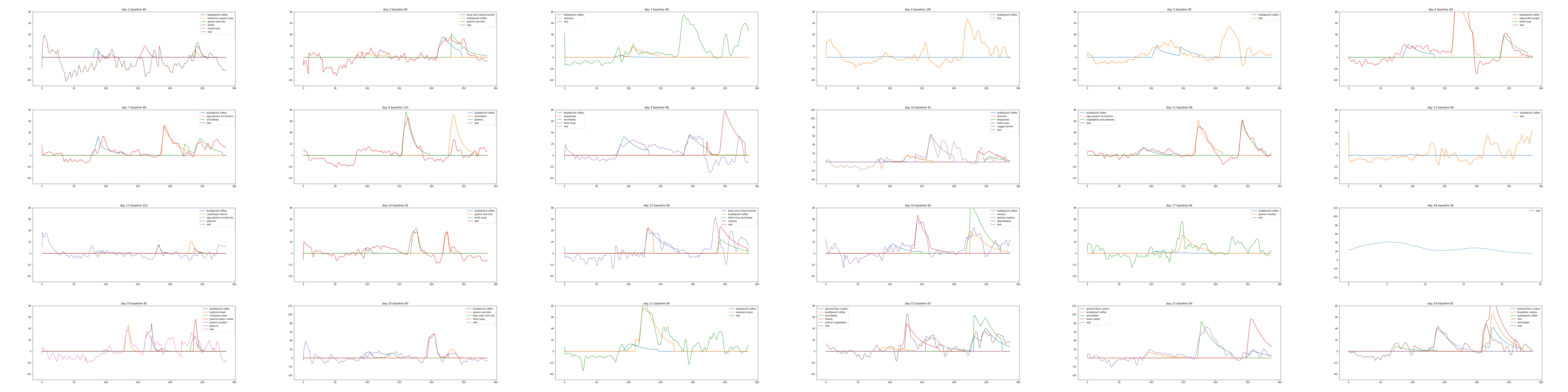
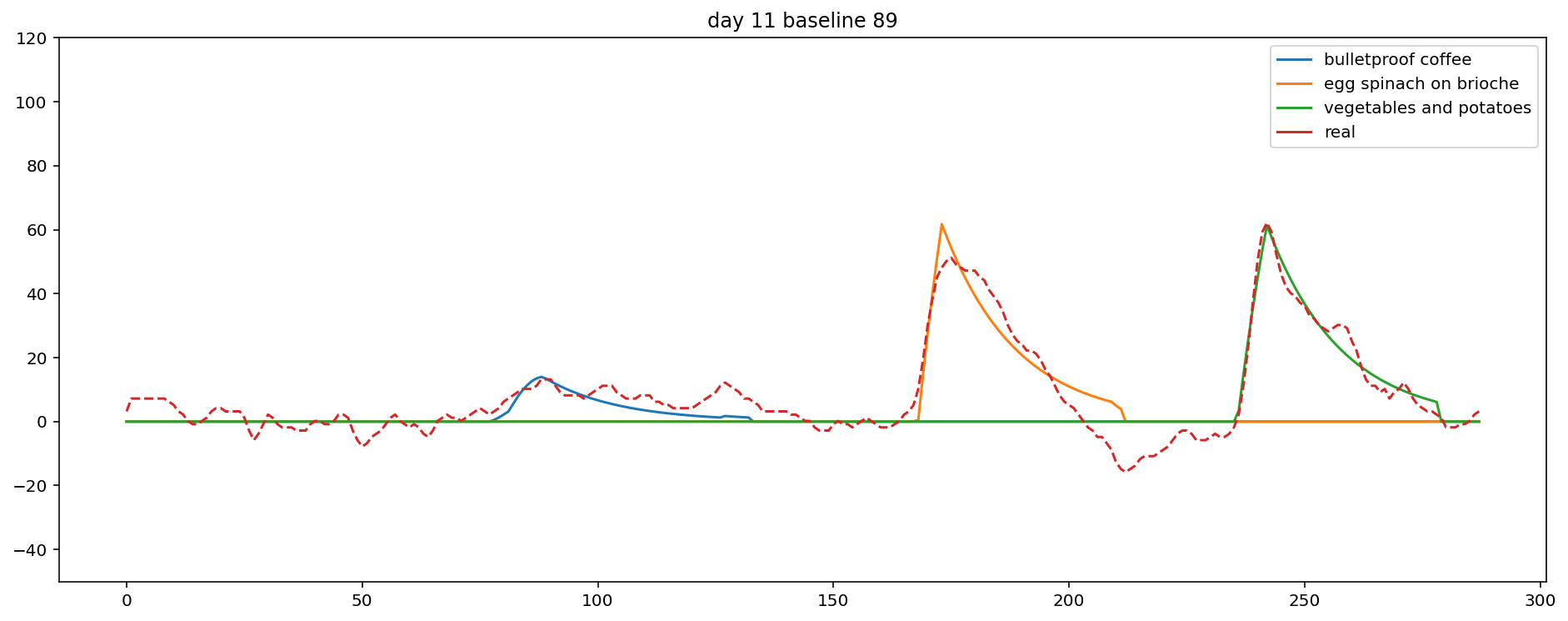
Plot results
Plotting the data in a sensible way is a little bit tricky.
Hopefully the plot is mostly self-explanatory,
but note that baseline is set to zero, the y-axis is on a log scale,
and the x-axis is midnight to midnight, in 5 minute increments.
def get_plot_sums(samples, bg_5min, hr_5min, fd_5min_key):
    samples = {k: onp.array(v) for k,v in samples.items()}
    bg_5min = onp.array(bg_5min)
    hr_5min = onp.array(hr_5min)

    means = []
    for n in tqdm(range(len(bg_5min))):
        means.append({"baseline": np.mean(samples[f"baseline_mu"])})
        for _j in range(MAX_TIMEPOINTS):
            for food in fd_5min_key:
                if f"add_{food}_{n-_j}_{_j}" in samples:
                    means[n][food] = np.mean(samples[f"add_{food}_{n-_j}_{_j}"])

    plot_data = []
    ordered_foods = ['baseline'] + sorted({k for d in means for k, v in d.items() if k != 'baseline'})
    for bg, d in zip(bg_5min, means):
        tot = 0
        plot_data.append([])
        for food in ordered_foods:
            if food in d and d[food] > 0.1:
                plot_data[-1].append(round(tot + float(d[food]), 2))
                if food != 'baseline':
                    tot += float(d[food])
            else:
                plot_data[-1].append(0)
    print("ordered_foods", ordered_foods)
    return pd.DataFrame(plot_data, columns=ordered_foods)
for n in DAYS:
    print(open(f"summary_{n}{SUB}.json").read())
    samples = json.load(open(f"samples_{n}{SUB}.json"))
    bg_5min = json.load(open(f"bg_5min_{n}{SUB}.json"))
    hr_5min = json.load(open(f"hr_5min_{n}{SUB}.json"))
    fd_5min = json.load(open(f"fd_5min_{n}{SUB}.json"))
    fd_5min_key = json.load(open(f"fd_5min_key_{n}.json"))

    print("fd_5min_key", fd_5min_key)
    plot_data = get_plot_sums(samples, bg_5min, hr_5min, fd_5min_key)
    plot_data['real'] = bg_5min
    plot_data['heartrate'] = [hr for hr in hr_5min]

    baseline = {int(i) for i in plot_data['baseline']}
    assert len(baseline) == 1
    baseline = list(baseline)[0]
    log_plot_data = plot_data.drop('baseline', axis=1)
    log_plot_data['real'] -= plot_data['baseline']

    display(log_plot_data);

    f, ax = plt.subplots(figsize=(16,6));
    ax = sns.lineplot(data=log_plot_data.rename(columns={"heartrate":"hr"})
                                        .drop('hr', axis=1),
                      dashes=False,
                      ax=ax);
    ax.set_ylim(-50, 120);
    ax.set_title(f"day {n} baseline {baseline}");
    ax.lines[len(log_plot_data.columns)-2].set_linestyle("--");
    f.savefig(f'food_model_{n}{SUB}.png');
    f.savefig(f'food_model_{n}{SUB}.svg');
Total blood glucose
Finally, I can rank each food by its total blood glucose contribution.
Usually, this matches expectations, and occasionally it's way off.
Here it looks pretty reasonable:
the largest meal by far contributed the largest total amount, and the milk chocolate had the shortest delay.
from pprint import pprint
print("### total grams of glucose")
pprint(sorted([(round(float(samples_1[food_type].mean()), 2), food_type) for food_type in samples_1 if "total" in food_type], reverse=True))
print("### food delays")
pprint(sorted([(round(float(samples_1[food_type].mean()), 2), food_type) for food_type in samples_1 if "delay" in food_type], reverse=True))
print("### food durations")
pprint(sorted([(round(float(samples_1[food_type].mean()), 2), food_type) for food_type in samples_1 if "duration" in food_type], reverse=True))
### total blood glucose contribution
[(123.52, 'food_g_total_vegetables and potatoes'),
 (84.24, 'food_g_total_egg spinach on brioche'),
 (79.69, 'food_g_total_milk chocolate'),
 (23.88, 'food_g_total_bulletproof coffee')]
### food delays
[(13.75, 'food_delay_egg spinach on brioche'),
 (12.03, 'food_delay_vegetables and potatoes'),
 (10.39, 'all_food_delay_mu'),
 (7.59, 'food_delay_bulletproof coffee'),
 (6.7, 'food_delay_milk chocolate')]
### food durations
[(11.42, 'food_duration_egg spinach on brioche'),
 (9.92, 'food_duration_bulletproof coffee'),
 (9.22, 'all_food_duration_mu'),
 (8.56, 'food_duration_vegetables and potatoes'),
 (7.01, 'food_duration_milk chocolate')]
Conclusions
It sort of works. For example, day 11 looks pretty good!
Unfortunately, when it's wrong, it can be pretty far off,
so I am not sure about the utility without imbuing the model with more robustness.
(For example, note that the r_hat is often out of range.)
The parameterization of the model is pretty unsatisfying.
To make the model hang together I have to constrain the priors to specific ranges.
I could probably grid-search the whole space pretty quickly to get to a maximum posterior here.
I think if I had a year of data instead of a month, this could get pretty interesting.
I would also need to figure out how to sample quicker, which should be possible given the simplicity of the model.
With the current implementation I am unable to sample even a month of data at once.
Finally, here is the complete set of plots I generated, to see the range of results.